
About this page
Numerical Weather Prediction (NWP),is a computer simulation of the atmosphere and the basis of all forecasts used by sailors.
Related pages
On this page -
- How the Atmosphere works
- Calculating it
- Operational forecasting
- Forecast Ensembles
- A future problem
- Climate models
Introduction
Weather forecasting is in its third phase.
- For thousands of years single observer forecasting was the only possible tool.
- From the late 1850s, the synoptic approach let forecasters "look" at the weather as plotted and analysed on charts. They learned how to interpret and predict but only in a subjective manner. There were some successes such as the D-Day forecast in June 1944 but many less good forecasts.
- The third phase is the era of large computing systems and satellite observing technologies. This has made possible the development of NWP.
How the Atmosphere Works
As �simply� as possible -
- Because it is very hot, the sun emits short wave radiation mainly as visible, UV and near-infrared light.
- Nearly 30% is reflected back out to space without warming the atmosphere.
- The remaining 70+% heats the earth and the atmosphere.
- Being much cooler, these radiate in infrared wavelengths.
- At some wavelengths this radiated heat goes direct out to space.
- At other wavelengths heat radiated by the earth is absorbed by greenhouse gases and then re-radiated to be absorbed by the ground and by greenhouses gases.
- Heat from the top of the atmosphere is radiated out to space.
- Heating and cooling of the earth varies with time of day, time of year, latitude and nature of the surface.
- Differential heating ----> temperatures differences ----> pressure differences ----> winds.
- Air movement ----> redistribution of pressure ----> changes in winds.
- Rising air ----> cooling.
- Descending air ----> warming.
- Contact with cold ground ----> cooling.
- Cooling ----> condensation ----> release of latent heat.
- Further cooling ----> freeze and -- more latent heat. These effects warm the air.
- Snow falling through warmer air melts ----> cooling. Rain falling through dry air evaporates ----> cooling.
- These latent heat effects ----> temperature change ----> pressure changes ----> wind changes.
- Cloud reflects solar radiation back out to space. Cloud absorbs radiation from the earth and re-radiates it back to earth and out to space.
- Some of the infra-red energy radiated by the earth is absorbed by greenhouse gases.
- Greenhouse gases radiate that heat back to earth and out to space
- Topography affects weather on all scales.
In schematic form:
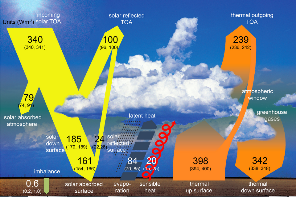
(From IPCC AR5, Woking Group 1 Final Report,)
All these processes can be expressed in mathematical equations and, in principle, be calculated. At the centre of these equations is one that says, in effect, that applying a net force to an object, including a parcel of air, results in change � acceleration or deceleration. This is Newton�s third law. There are always forces in the atmosphere � gravity, the Coriolis effect and pressure gradients. Consequently, there is always change. Pressure gradients are always changing so that the atmosphere is always in a state of flux.
Calculating it
Physicists describe weather forecasting as an initial value problem. At the initial time, T=0, these forces can be calculated. Therefore, the rates of change of each weather element can be calculated. That allows estimates to be made a short time, 4 minutes ahead for the Met Office global model, of winds, temperatures, pressures, water vapour and liquid water. These new values then provide a starting point to calculate for the next few minutes.
- Data analysis uncertainties.
The first problem is to determine the current conditions. There are many sources of data used in NWP. These have different characteristics in the way they represent the atmosphere. There are differences in accuracy, resolution, amount of data of various kinds and differences in times when the measurements were made. The process of data analysis uses a 4-dimensional mathematical process and is under continual review and experimentation. There is no definitive solution to the problem and there area be uncertainties in the analysis detail.
- Model Physics
Data and data analysis uncertainties have reduced largely because of improved satellite instrumentation. More significantly, there are uncertainties in evaluating the effects of heating by conduction, convection, radiation and latent heat. None can be calculated accurately. Many values are derived using a system known as "parameterisation", effectively, an intelligent guess based on studies of the atmosphere in widely different geographical and weather situations.
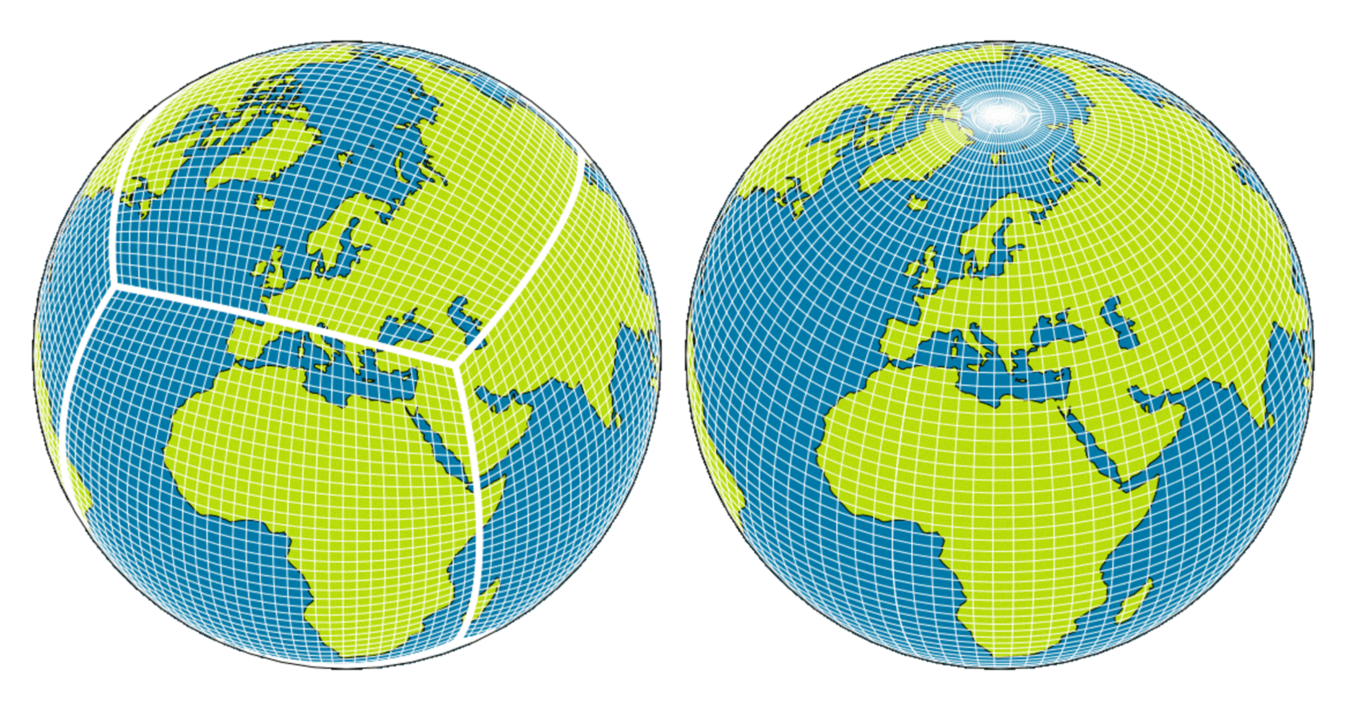
- Grids - global and limited area
An obvious model approximation is to represent the atmosphere by values on a 3-dimenional grid. The �traditional�, grid, as on the right side below, has obvious problems near the poles. There are various alternatives such as on the left side.
The UK Met Office global grid (2017) has a spacing of about 10 km, 0.1 degree lat/lon in the horizontal. There are 4,916,200 grid point with, 70 levels at each from about 20 m to 80 km above the surface of the earth. The Met Office uses a closer level spacing near the surface and jets stream, where there can be marked vertical gradients, and fewer at other levels.
Limited area models are �nested� in global models and, as seen here, do not have the same problem.
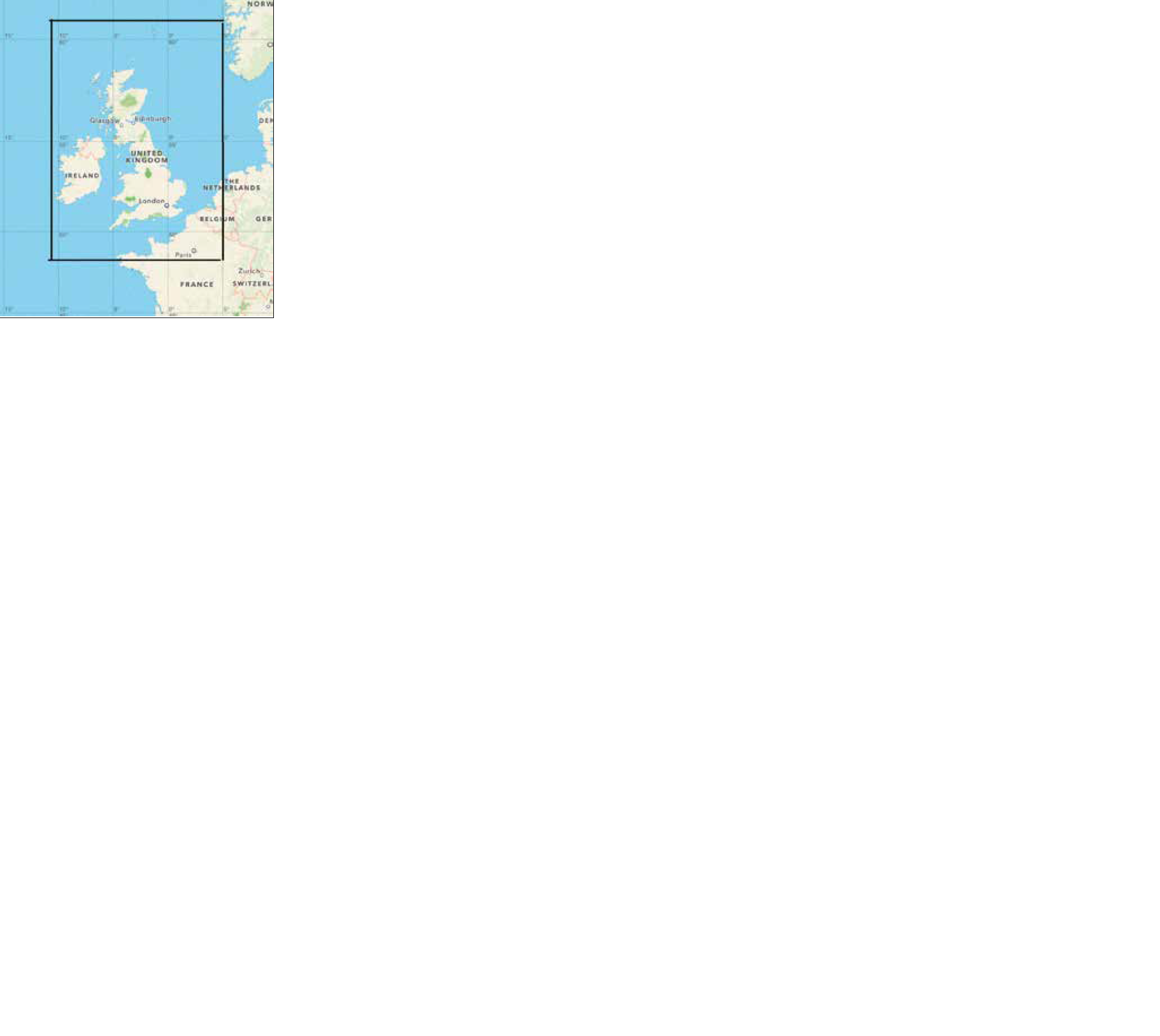
Nested within the Global model, the Met Office computes an area roughly 3000x3000 km wiyh a 4 km grid. Within that, they calculate on a 1.5 km grid for UKV. This is an area roughly 1000x1200 km covering the British Isles and surrounding waters,
- Effective resolutionStrong'''
My page on Model grids shows the problem of using a grid to describe geographical and atmospheric shapes. In addition, to the limitations of a grid point presentation, there is also the the uncertainties resulting from parameterisation of the physics. Models have to filter out small detail, otherwise spurious detail might grow unrealistically with the risk of model instability. As a result, any model can only resolve forecast data to about 4 or 5 grid lengths. This is the Effective Resolution.
This effective resolution has been known to modellers for many years but is ignored by third party providers who usually, wrongly, equate grid length with forecast resolution.
Operational forecasting
The UK Met Office runs its global NWP models on a 6-hourly basis. Forecasts for the first 6 hours of the last run are combined with all the observational data received over that period to produce the starting point for the next forecast.
In order to meet deadlines, there has to be a data cut-off time. Data arriving after that time are used later to re-compute the first 6 hours� forecast so getting the best start possible for the following run.
Limited area or meso-scale models are run in the same way using global model output to provide input around model boundaries. All this is on a �best endeavours� basis and users should always bear in mind the limitations to forecast accuracy.
Chaos and Forecast Ensembles
Chaos is always a problem although the idea that a single butterfly flapping its wings could lead to a major weather system is a rhetorical question taken out of context. In fact, it cannot but small disturbances can and often do grow into large ones. An mid latitude frontal system starts as a small wave on the polar front and hurricanes begin as groups of thunderstorms.
There are always uncertainties in detail of weather analyses. These lead to uncertainties in the deterministic forecast.
Model ensembles are a way of tackling this problem. After running the forecast model, small variations can be put into the analysis that are compatible with the original data. The forecast can be run many times and a spread of results obtained. The spread of these indicates the degree of uncertainty in the deterministic forecast.
A future problem
The amount of information that can be provided is enormous and access by users will become an increasing problem. How many sailors will have the ability to assess outputs from an ensemble? How many will want to spend the time needed to do so?
When will high speed communications become affordable for access over radio systems?
One thing is certain and that is that the written or spoken word will not and cannot cope with all the variations in the weather that exist, whether they are well forecast or not.
Annex - Computers
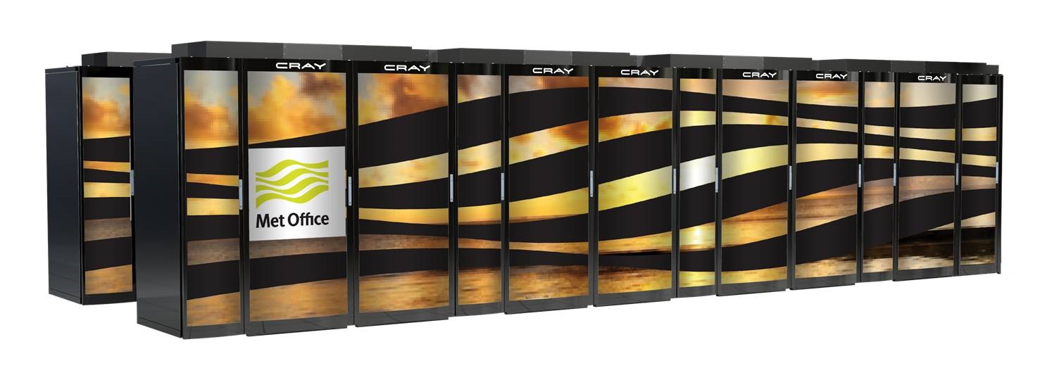
The atmosphere is, in effect a truly massive analogue computer of infinite complexity. Since the end of WW2, man has tried to simulate the atmosphere using a succession of digital computers of ever-increasing power. The latest Met Office computer was installed in 2017, a Cray XC40 can make 14,000 trillion calculations per second. It can hold 2 petaflops of memory and 24 petaflops of hard storage.
ECMWF installed the same computer but, 5 years alater, have now upgraded to an Atos HPCF, an even more powerful system. It has always been the case that, whenever they get a new computer, meteorologists are already specifying their next machine. With climate modelling, that is even more true.